Stock Price Prediction using Machine Learning with Python

Introduction

Stock price prediction is crucial for making informed investment decisions. With advancements in machine learning, we can leverage historical data to predict future stock trends. In this tutorial, we will walk you through how to use an LSTM model to predict Apple’s stock price.

Why Use LSTM for Stock Prediction?

LSTM is a special kind of Recurrent Neural Network (RNN) that can learn long-term dependencies. It’s ideal for time-series data like stock prices, which exhibit trends over time. LSTM can remember information for long periods, making it well-suited for stock market predictions.

Dataset and Libraries

We will use Yahoo Finance to download Apple’s stock price data from September 2019 to October 2020. You can install necessary libraries with the following:

pip install numpy pandas yfinance keras matplotlib scikit-learn

Importing Required Libraries:

import numpy as np
import pandas as pd
import yfinance as yf
from sklearn.preprocessing import MinMaxScaler
from keras.models import Sequential
from keras.layers import Dense, LSTM
import matplotlib.pyplot as plt

Step 1: Load the Dataset

We will fetch historical data for Apple (AAPL) stock using the yfinance library.

data = yf.download("AAPL", start='2019-09-10', end='2020-10-09')
data = data.filter(['Close'])
dataset = data.values

Step 2: Data Preprocessing

We scale the data using MinMaxScaler, which normalizes the dataset. We’ll also split the data into training (80%) and testing (20%) sets.

scaler = MinMaxScaler(feature_range=(0,1))
scaled_data = scaler.fit_transform(dataset)
training_data_len = int(np.ceil(len(dataset) * .8))

train_data = scaled_data[0:int(training_data_len), :]
x_train, y_train = [], []

for i in range(60, len(train_data)):
    x_train.append(train_data[i-60:i, 0])
    y_train.append(train_data[i, 0])

x_train, y_train = np.array(x_train), np.array(y_train)
x_train = np.reshape(x_train, (x_train.shape[0], x_train.shape[1], 1))

Step 3: Build the LSTM Model

The model consists of two LSTM layers, a Dense layer, and an output layer to predict the stock prices.

model = Sequential()
model.add(LSTM(50, return_sequences=True, input_shape=(x_train.shape[1], 1)))
model.add(LSTM(50, return_sequences=False))
model.add(Dense(25))
model.add(Dense(1))

model.compile(optimizer='adam', loss='mean_squared_error')
model.fit(x_train, y_train, batch_size=1, epochs=20)

Step 4: Testing the Model

For testing, we prepare the testing data by using the scaled values of the last 60 days of the training data.

test_data = scaled_data[training_data_len - 60: , :]
x_test, y_test = [], dataset[training_data_len:]

for i in range(60, len(test_data)):
    x_test.append(test_data[i-60:i, 0])

x_test = np.array(x_test)
x_test = np.reshape(x_test, (x_test.shape[0], x_test.shape[1], 1))

Step 5: Make Predictions

We use the trained model to predict the stock prices and then scale them back to the original form.

predictions = model.predict(x_test)
predictions = scaler.inverse_transform(predictions)

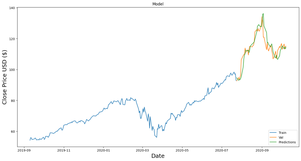
Step 6: Visualizing the Predictions

Finally, we visualize the actual vs. predicted stock prices using matplotlib.

train = data[:training_data_len]
valid = data[training_data_len:]
valid['Predictions'] = predictions

plt.figure(figsize=(16,8))
plt.title('Apple Stock Price Prediction Model')
plt.plot(train['Close'])
plt.plot(valid[['Close', 'Predictions']])
plt.xlabel('Date')
plt.ylabel('Close Price USD ($)')
plt.legend(['Train', 'Actual', 'Predicted'], loc='lower right')
plt.show()

Conclusion

In this tutorial, we used LSTM, a type of recurrent neural network, to predict stock prices based on historical data. While this model provides an interesting approach to time-series prediction, it’s important to note that stock prices are influenced by many external factors, making accurate prediction difficult. Always use machine learning predictions as part of a broader strategy when trading stocks.

Full code : github